SQL for accounting and finance professionals

If you’re an accounting or finance professional wanting to learn SQL, I’ve got good news: most of the knowledge you have of Excel or Google Sheets can be translated into SQL. Whether you’re looking at a spreadsheet or a database table, the core fundamentals are the same: it’s all about manipulating a big grid of data. This guide will show you how to query databases through comparisons to the tools you already know: spreadsheets.

Contents

• My two key principles
• Before we start
  • Tools
  • Using SQL in Access
  • Dataset
• Getting data from our table
  • Starting simple – one column
  • Getting more data with multiple columns
• Combining tables together
• Calculations in our table
  • Adding calculated columns
  • Grouping and summarizing data
• Filtering data from our table
  • Based on columns
  • Based on summarized data
• Sorting our data
• The order we write our SQL matters
• More resources

My two key principles

Lets start with two theories of mine which, if you’re willing to accept them, will make learning SQL dead simple.

1. Database tables are just spreadsheets in disguise

Just like spreadsheets, database tables are nothing more than a collection of rows and columns. Compare the two and you’ll notice that they are incredibly similar. Based on this, it’s pretty easy to move from thinking about data in spreadsheets to data in tables.

2. Writing code is just like asking a coworker to get some data from Excel for you

While writing code might be intimidating at first, all your doing is asking the database to get some data for you. This isn’t all that different than if you were training a new coworker and had to explain everything out loud to them. Just like explaining this to a coworker you need to specify:

1. What data you want to see
2. Where they should get the data from
3. What calculations they should perform on the data

SQL is largely based on plain English, so as long as you can communicate what you’re looking for to someone else you should be able to write the code you need.

Before we start

A few notes on the tools and data sources we’ll be using.

Tools

For the examples below I’m going to be working in Excel and Access since you likely already have these installed on your computer. That having been said the same concepts apply to other spreadsheet tools like Google Sheets and other database systems such as Google Cloud Platform, Oracle, or SQL Server.

The great thing about SQL is that its supported by nearly all database systems, so you only have to learn it once and you can keep using it no matter what database system you are using.

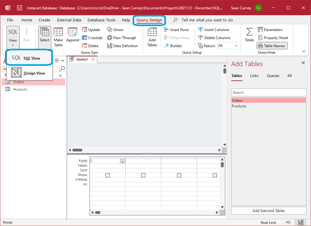
Using SQL in Access

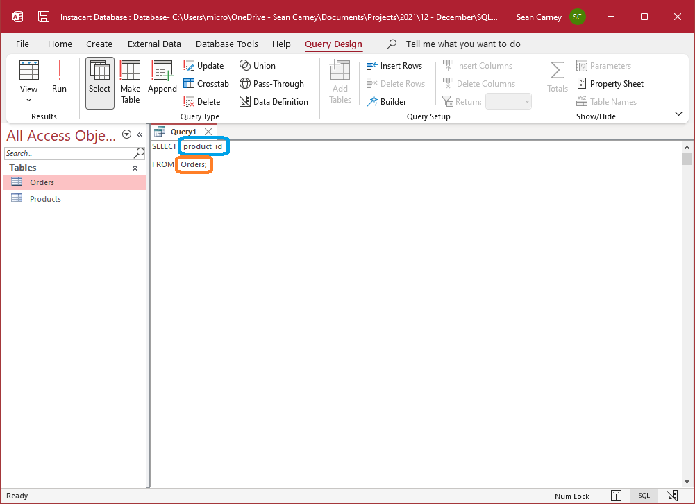
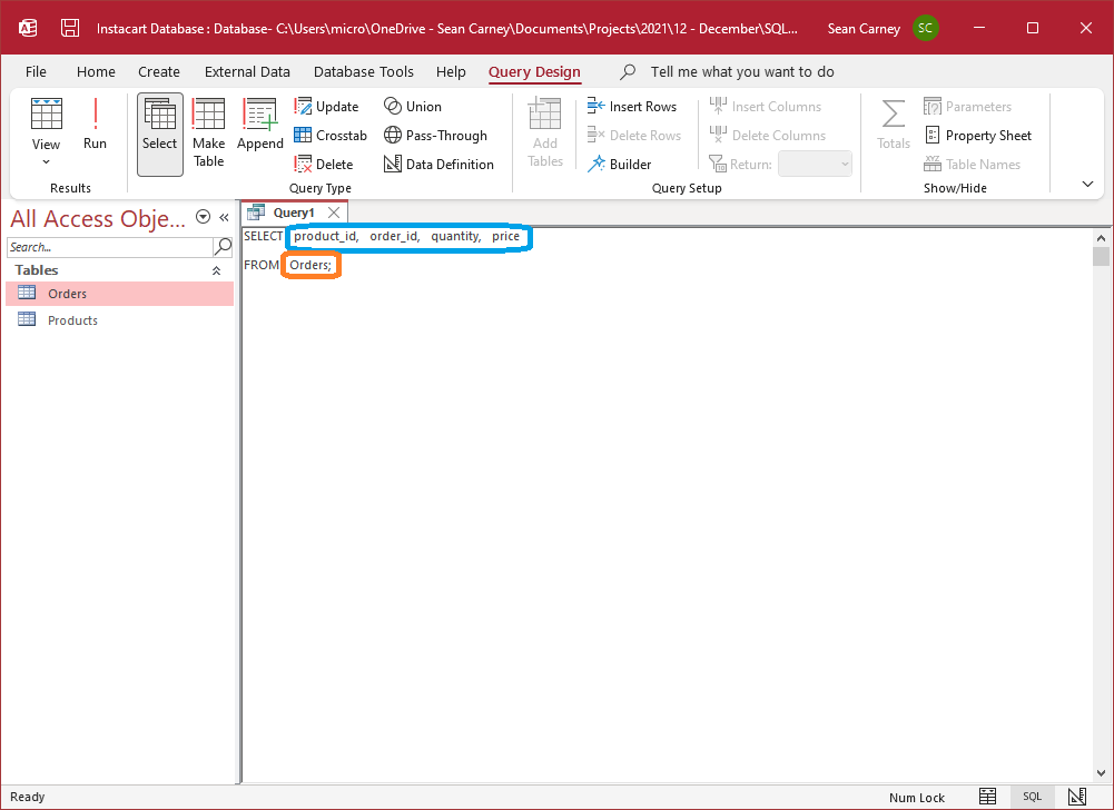
By default, when we try to create or edit a query in Access we’re presented with a visual query editor not SQL. To view the SQL, click on the top left icon on the Query Design ribbon and select SQL from the drop down which will appear.

Dataset

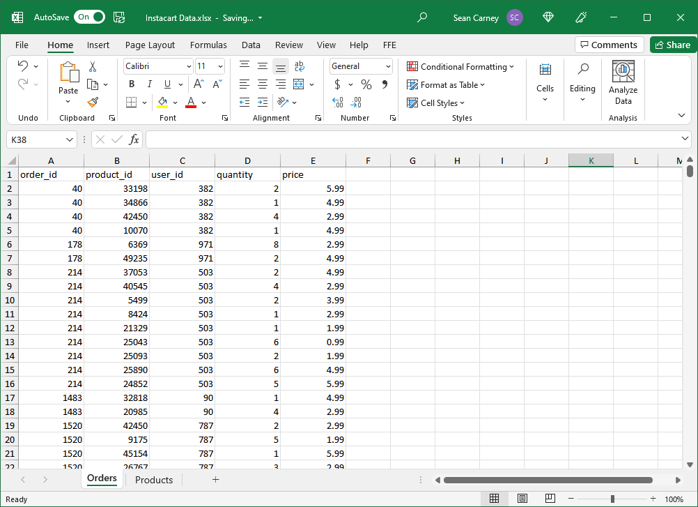
I’m going to use a bunch of demonstrations below based on 2017 Instacart purchases of groceries. Note that I’ve changed this data somewhat for the purposes of these examples by adding some order quantities and purchase prices to the data, and simplifying the product information.

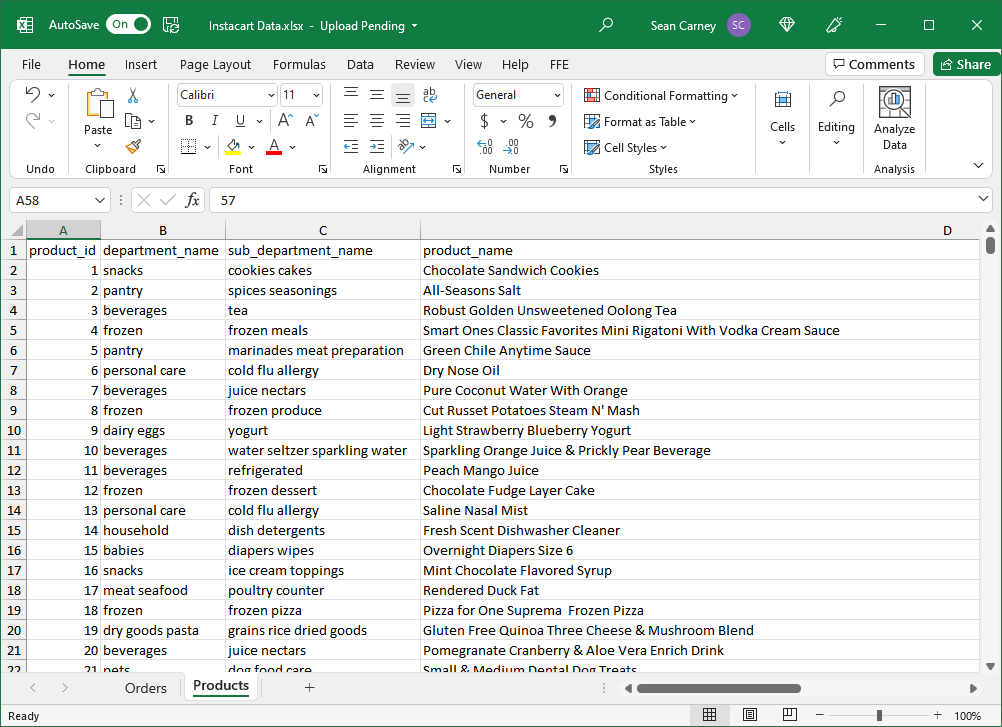
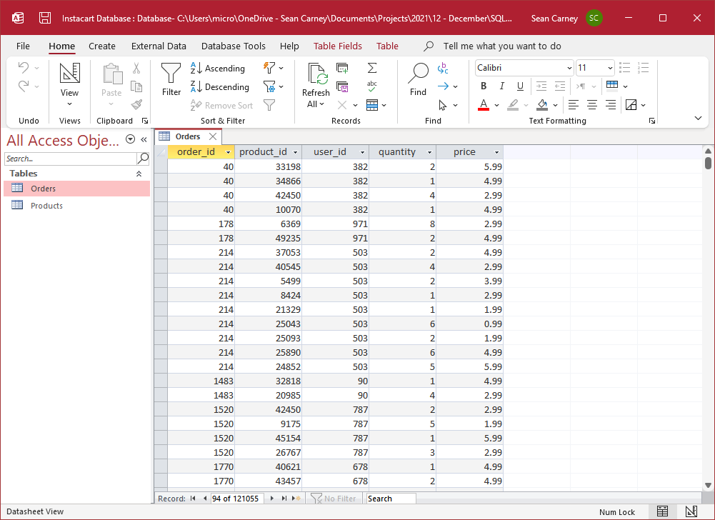
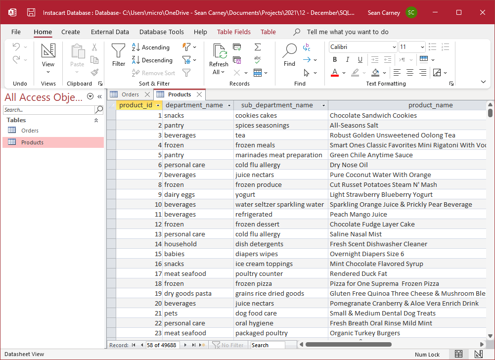
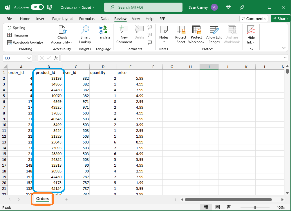
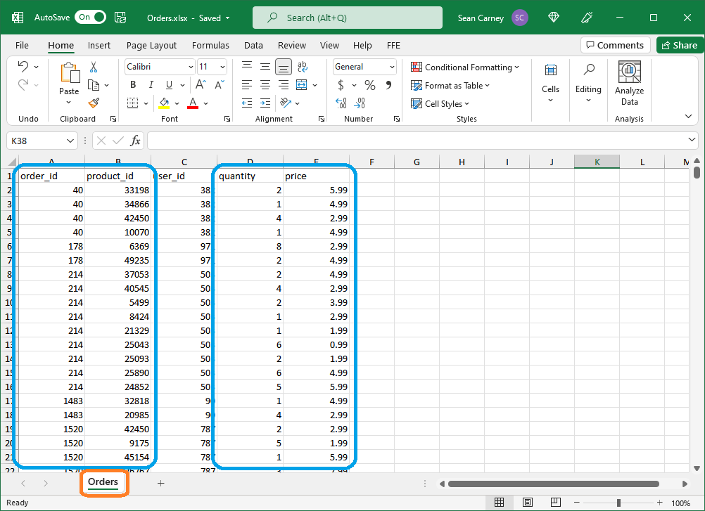
I’ll be working with two worksheets of data, one is a list of transactions and the other is a list of product details. The two lists are linked by a product_id field which is a unique identifier for the product sold. I’ve also dumped those exact same two worksheets into database tables so we can query them.

• 

• 

• 

• 

Getting data from our table

Starting simple – one column

Let’s get started by getting some data, say a list of the product numbers, from our list of grocery purchases.

In Excel we would do this by asking our coworker to:

Get me the column of “Product IDs” from the “Orders” worksheet.

Only instead we are going to do in code, and it looks like this:

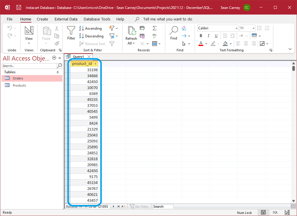
SELECT product_id
FROM Orders;

Writing the code actually uses less words than asking our coworker, but all the same meaning is there. We’re asking for a single column from the Orders spreadsheet. We ask for specific columns by “select-ing” them, and then say where the data should come from.

• 

• 

• 

Getting more data with multiple columns

Carrying this example on further, let’s say we want to see the product number, order number, quantity and price from the orders spreadsheet. We could ask our coworker:

Get me the “Product IDs” , “Order IDs”, “Quantity”, and “Price” from the “Orders” worksheet.

Or we could accomplish the exact same thing by writing the following SQL:

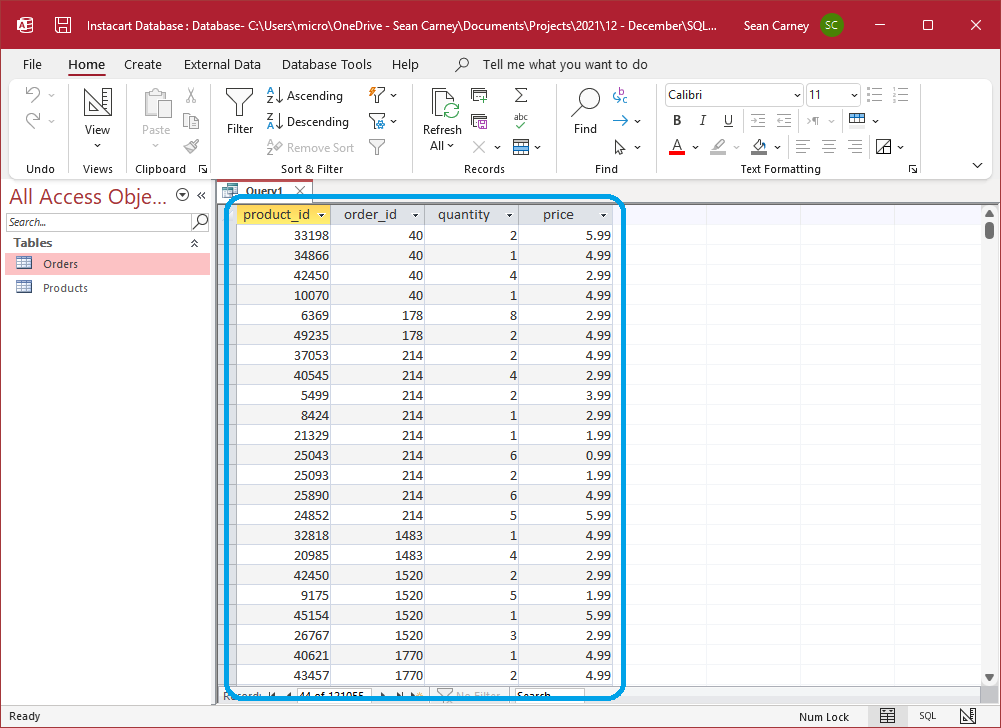
SELECT product_id, order_id, quantity, price
FROM Orders;

It’s just like before, we “select” the columns we want to see and provide the table where the data should come from, only this time we’re putting a comma between each of the column names since there’s more than one in our list.

• 

• 

• 

Combining tables together

The data we pulled in the example above isn’t very readable since we only included a product number. Let’s fix that by adding in some departments and product names.

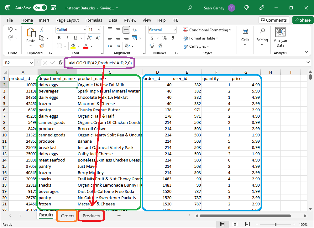
In Excel we’d typically accomplish this using either a =vlookup() on the product number or =index(match()). To describe this to our coworker, we’d likely say:

Get me the “Order IDs”, “Quantity”, and “Price” from the “Orders” worksheet, and add in the “Department Name” and “Product Name” from the “Products worksheet.

You can use the “Product ID” to link the orders and product information together.

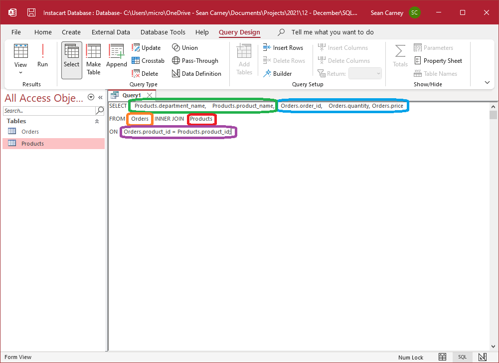
Now this same task can be done in SQL with:

SELECT Products.department_name, Products.product_name, Orders.order_id, Orders.quantity, Orders.price
FROM Orders INNER JOIN Products
ON Orders.product_id = Products.product_id;

You’ll see that a few things have changed in our SQL since the last example.

1. First, since we are now referencing multiple tables, we’ve prefixed our column names with the tables that those columns should come from.
2. Next, we’ve changed our FROM statement to include the other table name and we’ve specified that we want to use an INNER JOIN. This just means that we only want to show orders that have a matching product. If any orders don’t have a matching product, they’ll be hidden from the results.
3. Lastly, you’ll see we specified that the matching between the two tables should be done using the product numbers in both tables.

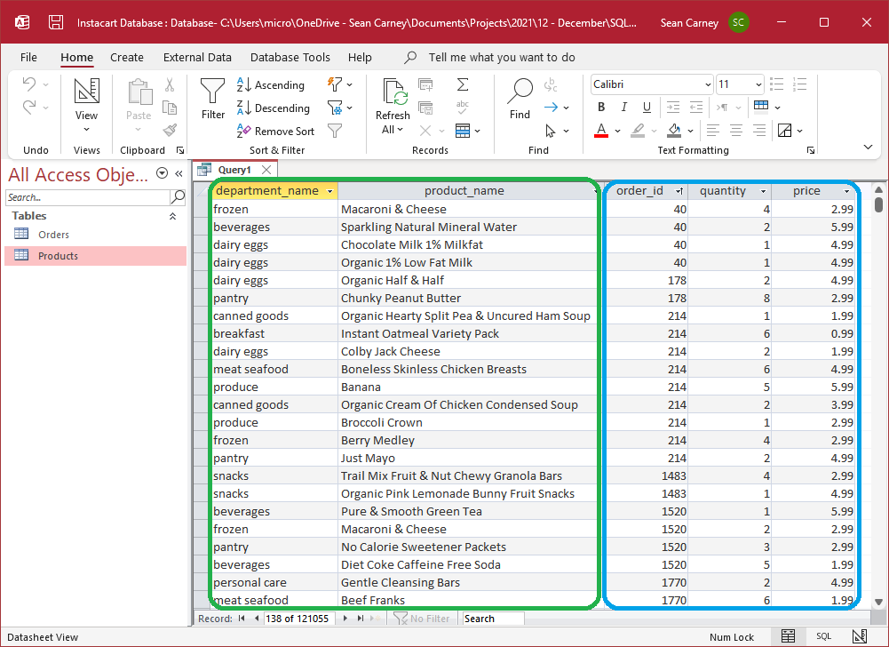
When we run this SQL (or write our vlookups in Excel) we get the exact same result:

• 

• 

• 

Calculations in our table

There’s two ways we can look at calculation, first by adding a new column with a calculation, or second by using a pivot table to group and summarize the data. We’ll go through each one with an example.

Adding calculated columns

Continuing our example before, we have a column with the quantity and a column with the unit price, but wouldn’t it be nice if we had a column with the extended price?

In Excel this is simple, we’d just put a formula in the following column to multiply the quantity and price together. To explain this to our co-worker, we’d likely say:

Get me the “Order IDs”, “Quantity”, and “Price” from the “Orders” worksheet, and add in the “Department Name” and “Product Name” from the “Products worksheet.

Add in a column for the extended price, by multiplying the “Quantity” and “Price”.

You can use the “Product ID” to link the orders and product information together.

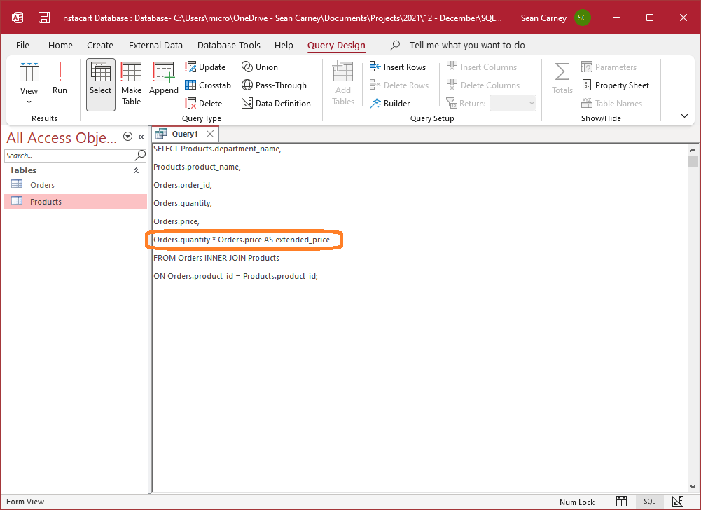
In SQL, the code for adding the extended price looks very similar to using a formula in Excel:

SELECT Products.department_name,
Products.product_name,
Orders.order_id,
Orders.quantity,
Orders.price,
Orders.quantity * Orders.price AS extended_price
FROM Orders INNER JOIN Products
ON Orders.product_id = Products.product_id;

There’s three things to note that we’ve added here:

1. The formula to create the extended price is as simple as multiplying the columns together in our SELECT statement.
2. We’ve renamed the column with our extended price by using AS followed by the column name we want. We can rename any of our columns by using this technique.
3. We’ve put some spacing between the column names with line-breaks to improve the readability. In SQL the line-breaks are ignored so we can add them liberally to make our code easier to read.

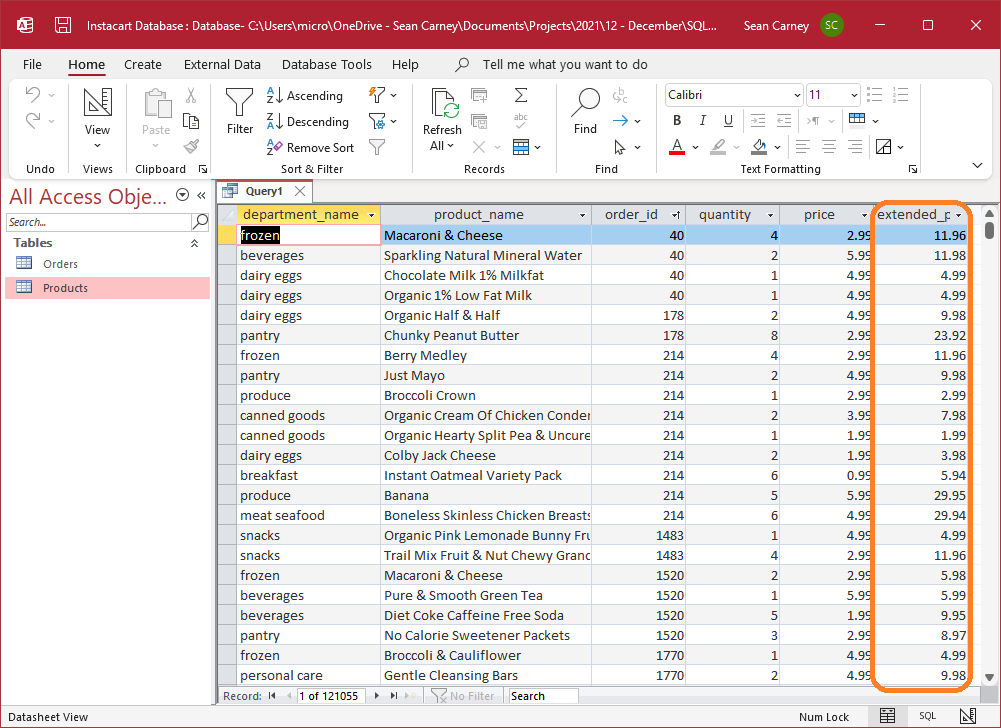
Here’s the result of doing this work, both in Excel and SQL:

• 

• 

• 

Grouping and summarizing data

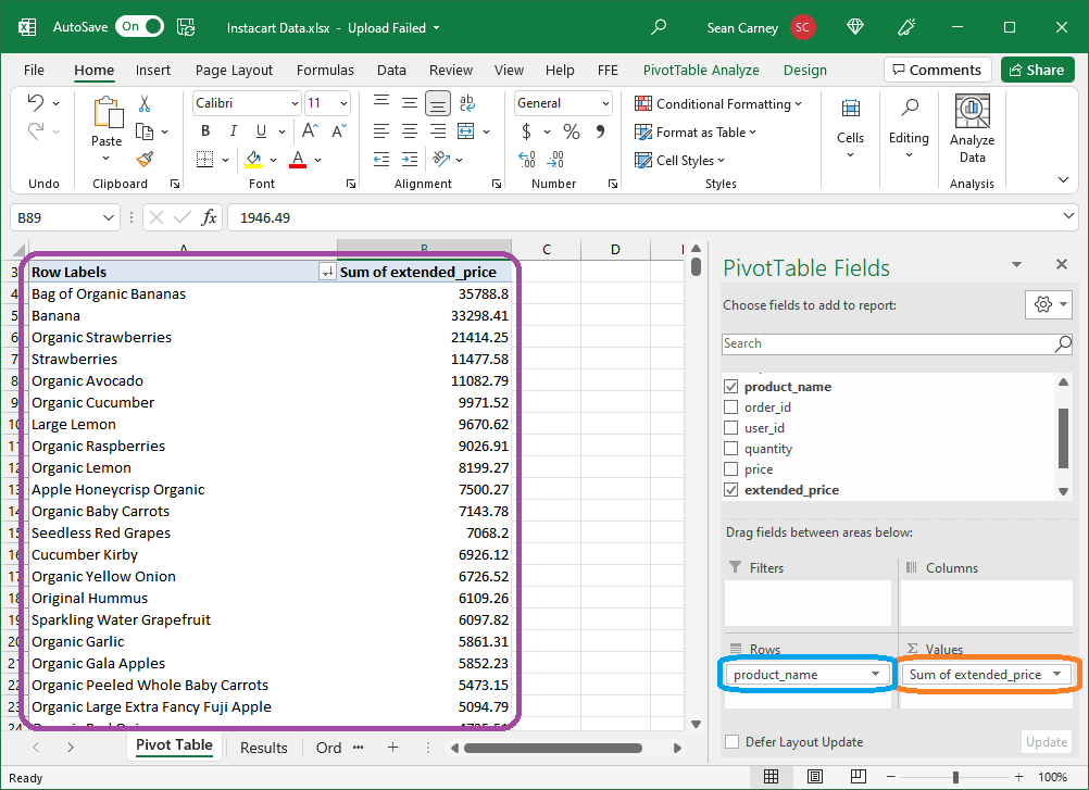
The other popular way to create calculations in Excel is by using pivot tables to create grouped and summarized data. Let’s say we wanted to see the total sales by product. We could ask our coworker:

Create a pivot table showing the “Product Name” from the “Products” worksheet and the total sales from the “Orders” worksheet. You’ll need to calculate the extended price first by multiplying the “Quantity” and “Price” from the “Orders” worksheet.

You can use the “Product ID” to link the orders and product information together.

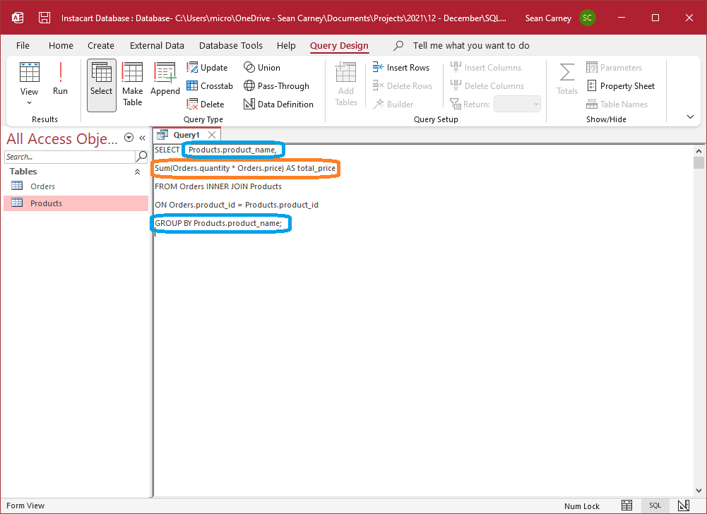
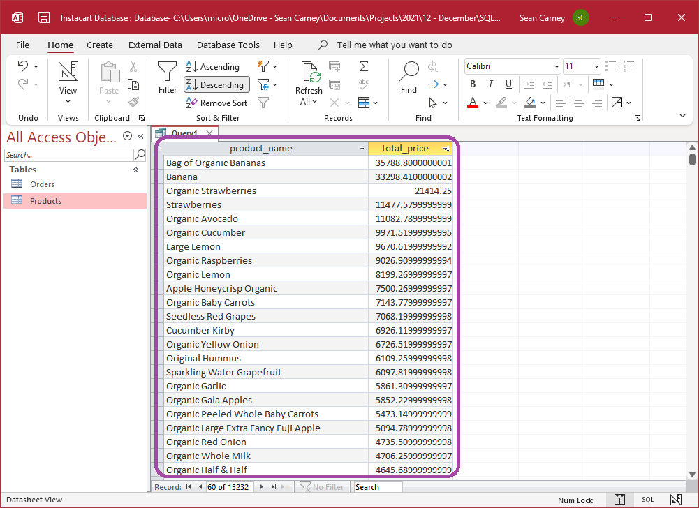
Now if we write this out in SQL, the code looks like this.

SELECT Products.product_name, 
SUM(Orders.quantity * Orders.price) AS total_price
FROM Orders INNER JOIN Products 
ON Orders.product_id = Products.product_id
GROUP BY Products.product_name;

Once again, our SQL code is shorter and simpler than the explanation to our coworker. Two key things to notice are:

1. We’ve accomplished the grouping and summarization by taking two actions. First we wrapped the extended price in a SUM() function to show that we want it added together. Next we’ve added a GROUP BY section at the end which says that we want the totals to show up by product.
2. The number of column names in the SELECT section has drastically reduced since our last example. Why is that? It’s because the SELECT is just the items we want to see on the screen. Since we only want two columns to display, we’ll only have two entries after SELECT.

• 

• 

• 

In addition to using SUM() to add values together, we can also use:

• MIN() to find the minimum value
• MAX() to find the maximum value
• AVG() to find the average value
• COUNT() to get the number of rows

Filtering data from our table

Another common task is to filter data, since sometimes we just want to see a subset of the results. We’ll look at two different examples, simple filtering based on column values and more complex filtering based on summarized values.

Based on columns

Just like using a filter in Excel, we can also filter data in SQL based on any of the cells in a row of data.

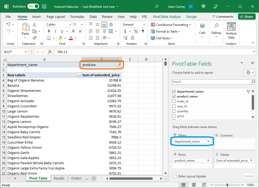
Continuing our example from before, let’s say that we want to see the total sales by product but limited only to the items from the ‘produce’ department of the store. To do this, we could ask our (very patient at this point) coworker to:

Create a pivot table showing the “Product Name” from the “Products” worksheet and the total sales from the “Orders” worksheet. You’ll need to calculate the extended price first by multiplying the “Quantity” and “Price” from the “Orders” worksheet.

You can use the “Product ID” to link the orders and product information together.

Once you’ve done that, filter the data to only show items from the “Produce” department.

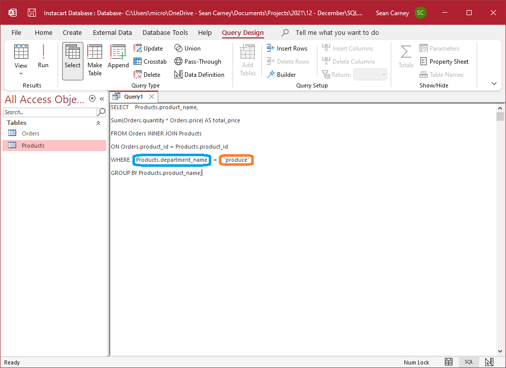
Or we could write the following SQL to accomplish the same thing:

SELECT Products.product_name, 
SUM(Orders.quantity * Orders.price) AS total_price
FROM Orders INNER JOIN Products 
ON Orders.product_id = Products.product_id
WHERE Products.department_name = "produce"
GROUP BY Products.product_name;

Notice all we added to the last example was an additional line starting with WHERE. We can use WHERE to filter based on the values in any of our columns. In this example we said we want to only show items where the department equals produce, but we can also use this on numerical values and using comparisons like greater than, less than, not equal to, etc.

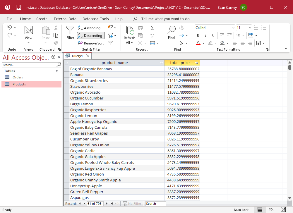
Here’s the output in Excel and Access of the example above:

• 

• 

• 

If we want to, we can also filter based on multiple columns by adding additional comparisons and using the words AND and OR to specify how the different comparisons should be combined. A quick example of this would be modifying the query above to only show items within produce with a price of at least 2.99:

SELECT Products.product_name, 
SUM(Orders.quantity * Orders.price) AS total_price
FROM Orders INNER JOIN Products 
ON Orders.product_id = Products.product_id
WHERE Products.department_name = "produce"
AND Orders.price >= 2.99
GROUP BY Products.product_name;

Based on summarized data

In addition to filtering based on the values of individual cells, we can also filter on aggregates (meaning the values of our SUM(), AVG(), COUNT() functions). A good example of this would be finding the products within produce that had sales exceeding $6,000.

Once again, we’d probably explain this to a coworker by saying:

Create a pivot table showing the “Product Name” from the “Products” worksheet and the total sales from the “Orders” worksheet. You’ll need to calculate the extended price first by multiplying the “Quantity” and “Price” from the “Orders” worksheet.

You can use the “Product ID” to link the orders and product information together.

Once you’ve done that, filter the data to only show items from the “Produce” department with total sales over $6,000

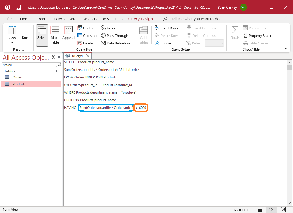
In SQL we could do the same thing by:

SELECT Products.product_name, 
SUM(Orders.quantity * Orders.price) AS total_price
FROM Orders INNER JOIN Products 
ON Orders.product_id = Products.product_id
WHERE Products.department_name = "produce"
GROUP BY Products.product_name
HAVING SUM(Orders.quantity * Orders.price) > 6000

Since we’re filtering based on aggregated data, instead of adding this additional request to our WHERE statement, we need to add this to the HAVING statement. Just like the WHERE statement, we can have multiple conditions separated with AND and OR, but each of the items we’re filtering on using HAVING should be an aggregate function like SUM(), AVG(), or COUNT().

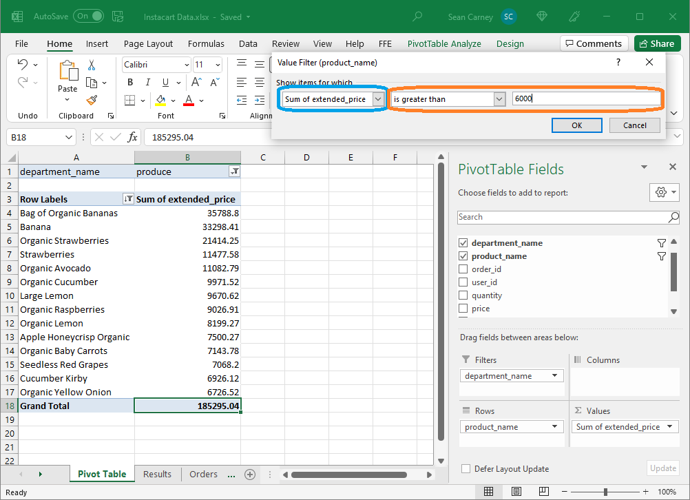
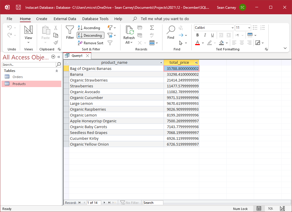
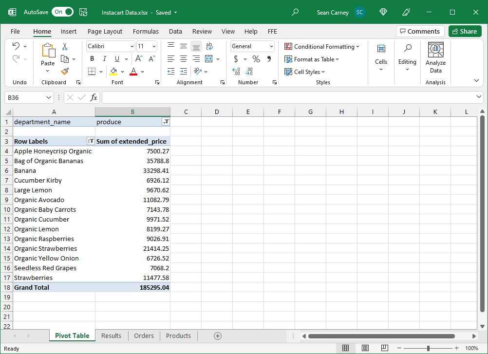
Here’s what this looks like in both Excel (using a value filter in the pivot table) and Access:

• 

• 

• 

Sorting our data

Lastly, let’s say that we want to sort our data. An example is sorting the results of our last example by product name.

We could ask our coworker to do this by:

Create a pivot table showing the “Product Name” from the “Products” worksheet and the total sales from the “Orders” worksheet. You’ll need to calculate the extended price first by multiplying the “Quantity” and “Price” from the “Orders” worksheet.

You can use the “Product ID” to link the orders and product information together.

Once you’ve done that, filter the data to only show items from the “Produce” department with total sales over $6,000, and sort the results by product name from A to Z.

To do this in SQL, instead we would type the following as our query:

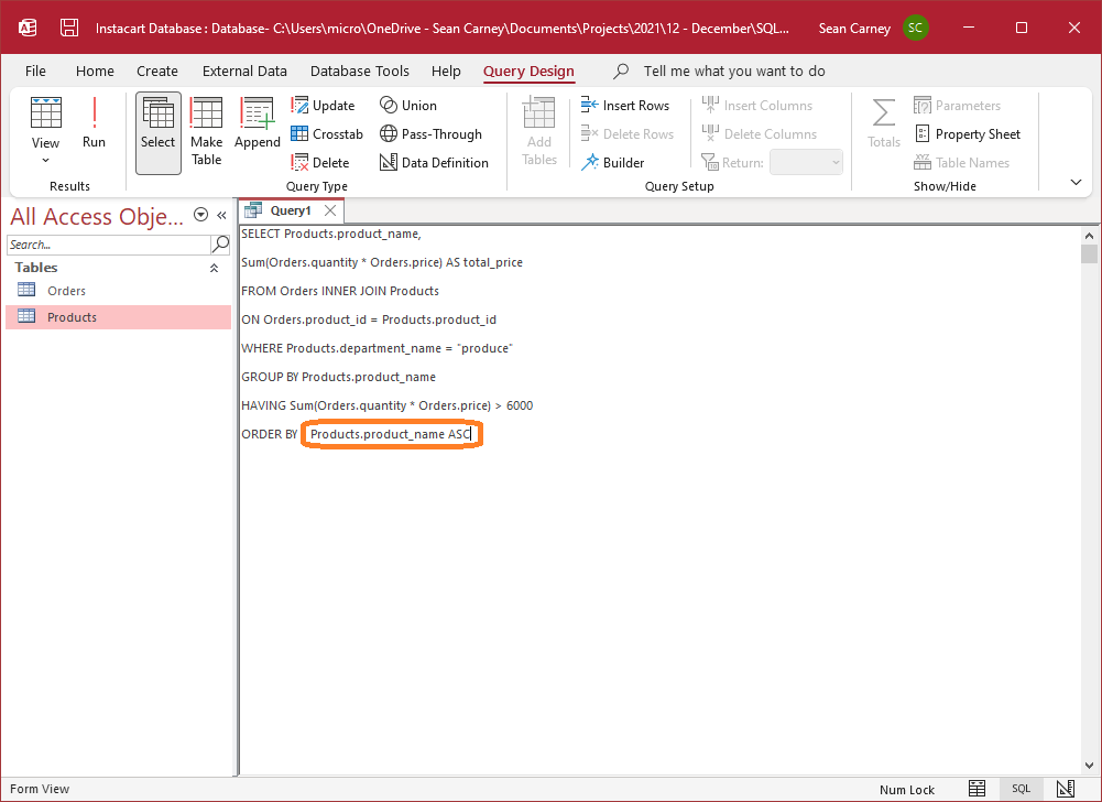
SELECT Products.product_name, 
SUM(Orders.quantity * Orders.price) AS total_price
FROM Orders INNER JOIN Products 
ON Orders.product_id = Products.product_id
WHERE Products.department_name = "produce"
GROUP BY Products.product_name
HAVING SUM(Orders.quantity * Orders.price) > 6000
ORDER BY Products.product_name ASC

To actually do the sorting, we’ve added ORDER BY to the end of the query with the field that we want to order by and the direction to sort the data. There are two direction abbreviations we can use:

• ASC which stands for ascending and sorts the data from A to Z or 0 to 9
• DESC which stands for descending and sorts the data from Z to A or 9 to 0

We can also sort by multiple columns by adding a comma and then the next column to sort by along with the direction that we want it sorted.

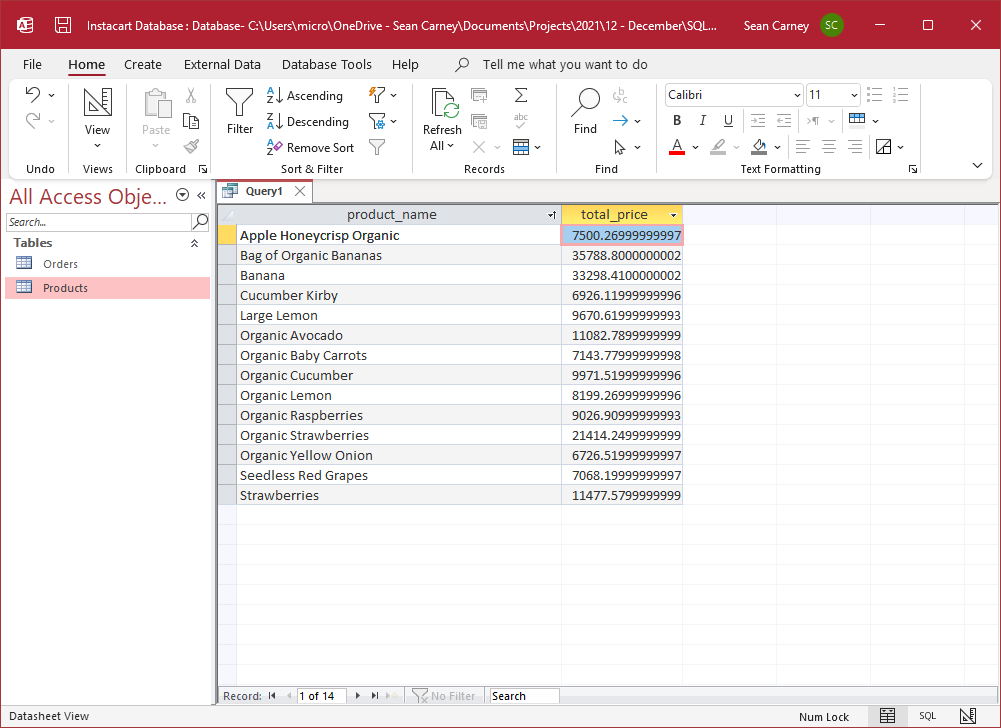
Here’s what this example looks like in both Excel (using a sorted column in our pivot table) and Access:

• 

• 

• 

The order we write our SQL matters

Before we end this, there’s one thing we’ve implicitly been doing but haven’t explained in detail yet: when we’re writing SQL, the order of the statements matters. Our database is expecting to see a query that is in this order:

SELECT ...
FROM ...
WHERE ...
GROUP BY ...
HAVING ...
ORDER BY ...

If, for some reason, we write a query where we start with FROM and then SELECT our columns, the query will fail with an error since the database always expects SELECT to come first and FROM to come second. Don’t get creative with the ordering.

More resources

This guide serves as a quick introduction to SQL by using Excel based examples, but there is a lot that wasn’t covered. I recommend that you import some Excel data into Access and try writing some SQL queries yourself to see how this works and get some practise.

For an overview of all the components of a SQL query, check out my SQL cheat sheet.

If you want to continue learning about SQL, topics to explore next would be working with more tables, different join types, using sub-queries, and analytic functions (which sadly aren’t available in Access).

Please leave a comment below to let me know if you found this helpful or have any questions.