One of the best ways to understand data is through the use of descriptive statistics, figuring out the minimum and maximum values, the median value, and the quartiles. When you’re working with smaller datasets this is easy, but with larger datasets you need to parse a lot of data to get these metrics. Luckily, you can use SQL to get descriptive statistics for your data directly from the database.
Contents
Background and source data
My goal is to get the minimum, 1st quartile, median, 3rd quartile, and maximum property values for each neighborhood / community in Calgary. To get the raw data, I’m going to be working with property assessment values from the City of Calgary’s open data portal. Based on the link above, you can download the assessed property value for each address within the city. The data also contains the community name for each address so we have an idea which neighborhood each property is in.
Here’s a sample of the raw data:
| CommunityName | Address | AssessedValue |
|---|---|---|
| AUBURN BAY | 535 AUBURN BAY HT SE | 441,000 |
| AUBURN BAY | 531 AUBURN BAY HT SE | 447,000 |
| AUBURN BAY | 527 AUBURN BAY HT SE | 380,000 |
| AUBURN BAY | 5 AUBURN BAY PA SE | 496,000 |
| AUBURN BAY | 9 AUBURN BAY PA SE | 470,500 |
| BEDDINGTON HEIGHTS | 48 BEACONSFIELD RD NW | 295,000 |
| BEDDINGTON HEIGHTS | 52 BEACONSFIELD RD NW | 379,000 |
| BEDDINGTON HEIGHTS | 1419 BERKLEY DR NW | 289,500 |
| BEDDINGTON HEIGHTS | 1417 BERKLEY DR NW | 331,000 |
| BEDDINGTON HEIGHTS | 1415 BERKLEY DR NW | 313,000 |
Tutorial
I’m going to approach this in two steps. First, I’m going to write a subquery which assigns each address to a quartile based on it’s community. After that, I’ll write another query which will take this data and summarize it by community.
Step 1: Using a query to assign quartiles to data
Let’s start with the subquery. Using SQL’s analytic functions and NTILE() we can assign each address to a quartile based on it’s community. This is pretty simple in code:
SELECT
	-- Get the community name
	CommunityName,
	-- Get the assessed value
	AssessedValue,
	-- Bucket the assessed value for each property into quartiles based on its community
	NTILE(4) OVER (PARTITION BY Community.Community ORDER BY AssessedValue) AS Quartile
FROM
	Assessments
Running this query results in one row for each property, showing the community name, assessed property value, and the quartile (based on the assessed property value) for that community:
| CommunityName | AssessedValue | Quartile |
|---|---|---|
| AUBURN BAY | 254,000 | 1 |
| AUBURN BAY | 254,000 | 1 |
| AUBURN BAY | 254,000 | 1 |
| AUBURN BAY | 254,000 | 2 |
| AUBURN BAY | 254,000 | 2 |
| BEDDINGTON HEIGHTS | 384,500 | 3 |
| BEDDINGTON HEIGHTS | 385,000 | 3 |
| BEDDINGTON HEIGHTS | 385,000 | 3 |
| BEDDINGTON HEIGHTS | 385,000 | 4 |
| BEDDINGTON HEIGHTS | 385,000 | 4 |
Step 2: Summarizing the quartile data by grouping
Now we need to summarize this by community. To do that, we’ll group by the community, use MIN() and MAX() to get the upper / lower boundaries of each quartile, and we’ll use CASE to pull each quartile into it’s own column. The full, final query to do this is:
SELECT
-- Show the community name
CommunityName,
-- Get the minimum value for the community
MIN(AssessedValue) Minimum,
-- Get the 1st quartile boundary for the community, which is the highest value in the 1st quartile
MAX(CASE WHEN Quartile = 1 THEN AssessedValue END) 1Quartile,
-- Get the median for the community, which is the highest value in the 2nd quartile
MAX(CASE WHEN Quartile = 2 THEN AssessedValue END) Median,
-- Get the 3rd quartile boundary for the community, which is the highest value in the 3rd quartile
MAX(CASE WHEN Quartile = 3 THEN AssessedValue END) 3Quartile,
-- Get the maximum value for the community
MAX(AssessedValue) Maximum,
-- Get a count of the total properties in the community
COUNT(Quartile) AS Count
FROM (
SELECT
-- Get the community name
Community.CommunityName,
-- Get the assessed value
AssessedValue,
-- Bucket the assessed value for each property into quartiles based on its community
NTILE(4) OVER (PARTITION BY Community.Community ORDER BY AssessedValue) AS Quartile
FROM
Assessments
) Vals
GROUP BY
CommunityName
ORDER BY
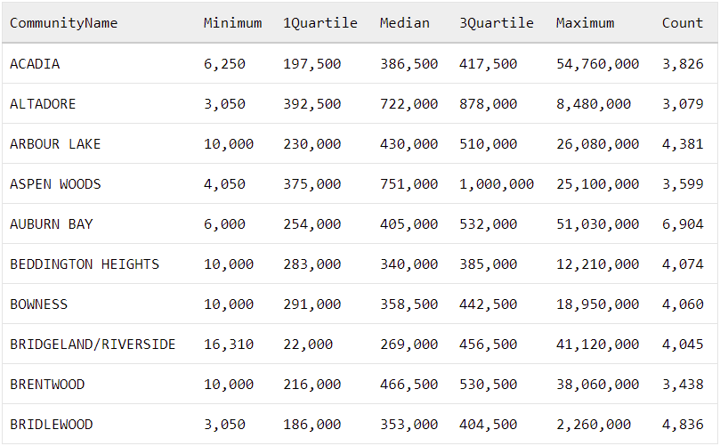
CommunityNameThere we go! When we run this query, it provides the descriptive statistics for each community as a single row, with the statistics running across the columns like this:
| CommunityName | Minimum | 1Quartile | Median | 3Quartile | Maximum | Count |
|---|---|---|---|---|---|---|
| ACADIA | 6,250 | 197,500 | 386,500 | 417,500 | 54,760,000 | 3,826 |
| ALTADORE | 3,050 | 392,500 | 722,000 | 878,000 | 8,480,000 | 3,079 |
| ARBOUR LAKE | 10,000 | 230,000 | 430,000 | 510,000 | 26,080,000 | 4,381 |
| ASPEN WOODS | 4,050 | 375,000 | 751,000 | 1,000,000 | 25,100,000 | 3,599 |
| AUBURN BAY | 6,000 | 254,000 | 405,000 | 532,000 | 51,030,000 | 6,904 |
| BEDDINGTON HEIGHTS | 10,000 | 283,000 | 340,000 | 385,000 | 12,210,000 | 4,074 |
| BOWNESS | 10,000 | 291,000 | 358,500 | 442,500 | 18,950,000 | 4,060 |
| BRIDGELAND/RIVERSIDE | 16,310 | 22,000 | 269,000 | 456,500 | 41,120,000 | 4,045 |
| BRENTWOOD | 10,000 | 216,000 | 466,500 | 530,500 | 38,060,000 | 3,438 |
| BRIDLEWOOD | 3,050 | 186,000 | 353,000 | 404,500 | 2,260,000 | 4,836 |
What next
Now that you can calculate the min, max, median, and quartiles by group in SQL, it’s easy to have a look at the data across different dimensions and get a feel for the distribution. While I grouped by the community above in the example, if the data had other dimensions such as “number of bedrooms” or “number of bathrooms” I could quickly change the query to get an overview of how those factors impacted the distribution of property values.
Try using this query to explore your data and see what insights you can uncover. If you find something interesting, I’d love to hear about it in the comments below.
Leave a Reply